

About the author

Silvio de Almeida Basques
Author of materials on internal quality control and information systems for laboratories.
Training and experience
Doctor, with residency and postgraduate degree from the Federal University of Minas Gerais and specialist title from the Brazilian Society of Clinical Pathology. Retired professor at the UFMG Faculty of Medicine.
Introduction

Dr. José Carlos de A. Basques
1941–2009
Several people who preceded us worked hard and became followers in the task of contributing to the study and actions for quality in clinical laboratories. We are very grateful to these professionals and we especially honor the memory of Dr. José Carlos by Almeida Basques, who worked brilliantly and was recognized throughout Brazil, among other works developed in his life, for his enthusiastic lectures, courses, conferences and the like, on the topic of Quality Control1,9.
Tribute to Dr. JCABasques
Em uma época de pioneirismo da Patologia Clínica, seu espírito empírico guiou-o para a área laboratorial, primeiramente no laboratório do Hospital do IPSEMG e também com o Dr. Orion de Bastos, seu sócio na Hemoclínica. Given the need to produce reagents "in house", he voluntarily attended the IPSEMG Laboratory on Saturdays to prepare the reagents to be used in the chemistry sector, together with Dr. Geraldo Lustosa Cabral, another great partner of his. Da otimização desses procedimentos e metodologias formou-se o embrião do que viria a ser a Labtest, uma das primeiras empresas nacionais em reagentes para laboratório e hoje entre as maiores da América Latina, motivo de grande satisfação para si. Dr. José Carlos was a scholar of quality control in clinical laboratories.
There is no force greater than that of an idea, whose time has come.— Victor Hugo
Nós entendemos que a qualidade dos resultados é uma responsabilidade dos profissionais do laboratório clínico, nos seus diferentes papeis. The director has the task of establishing and leading his laboratory in the big picture, assuming this responsibility and translating it into the implementation of Quality Management. Deve cuidar do atendimento às normas legais (ANVISA Technical Regulation), do atendimento aos requisitos dos programas de acreditação e disponibilização de instrumentos, insumos e ferramentas adequados para o melhor desempenho do setor analítico. Professional analysts also have an important role to play
to gain in-depth knowledge of analytical systems, operational standards and statistical process control. Coordinated actions at these two main levels enable the creation and implementation of the best Quality Management (GDQ).
We all learned and recognized that Quality Management is a complex set of actions, which are based on planning, implementation, control and re-elaboration of processes for continuous quality gains. The scope we seek to address in this and other of our articles refers to the control of analytical processes, which is only part of GDQ. Our intention is to disseminate the need to carry out GDQ, which can initially be done through Internal Quality Control, in Statistical Process Control. Until then, a very widespread paradigm in our country is that if the laboratory carries out External Control through Proficiency Tests, it would guarantee the quality of its analyses. "This procedure, in addition to not being sufficient to add quality to laboratory processes, has the serious limitation of not carrying out daily verification of results. As evaluation results take a long time to return to program participants, process control procedures are no longer effective because, when corrective actions are implemented, many defective results may have been released." We understand
that participation in Proficiency Testing Programs is essential, but it is not enough.
Quando há 14 anos lançamos um software para o Controle Interno da Qualidade acreditávamos no seu valor como ferramenta de auxílio em uma dessas etapas, mas que não dispensava outras ações, mesmo anteriores, de planejamento e revisões para o IQC, bem como de participação do laboratório em ensaios de proficiência, ou seja, a External Quality Assessment.
We believe laboratories should have practical, effective tools to make quality control indicators tangible, bridging the gap between their daily work and the modern quality assessment methods available.
Quality Management Steps
There are different approaches to understanding and planning actions for quality. Todas as definições da qualidade podem ser interpretadas, no campo de atuação do laboratório clínico, como sendo o estabelecimento de condições para que todos os testes realizados auxiliem os clínicos na prática da excelência da medicina9.
Modern quality management methods involve much more than statistical process control. Good laboratory practice, quality assurance, quality improvement and quality planning are also essential components of quality management9,10.
In a general and very simplified overview of how we are going to take care here,
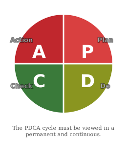
we can summarize this approach in the well-known cycle PDCA, acronym that comes from English Plan, Do, Check, Action, ou seja, Planejar, Executar, Controlar e Agir. This cycle is well known in society and by everyone who has ever worked with organizational development and implementation of quality systems. The beginning is always with planning.
The laboratory must then take care of at least these four management steps, which can be a good start. Adding other actions, for example, for the pre-analytical phase, will make the path to quality more accurate and customers will be better served.
These introductory words are important so that new students of the subject realize that here in this article we will cover just one stage of Quality Management, applying statistical methods there. In PDCA this step corresponds to Control (Check) which, as you can see in the diagram, is the third in the process. With this, we reaffirm that Internal Quality Control, although very important, is not the entirety of the actions that laboratory professionals must be concerned with to guarantee quality in their work.
Statistical Quality Control
Statistical Quality Control procedures are used in all branches of activity. In clinical laboratories, they are established to monitor the analytical performance of a system and alert professionals to the occurrence of problems that could compromise the usefulness of patient test results for medical purposes. In the PDCA cycle it corresponds to the third stage, or phase. This type of control is the "dream" of different organizational managers, who would like to have measurement systems and collection of indicators to assess their control status and quality. Clinical laboratories already have this facility, with IQC methods.
Work in clinical laboratories with analyzes that provide quantitative and other qualitative data. For those of the first type, statistics made a great contribution to the establishment of methodologies for controlling analysis processes. The use of appropriate control methods, implemented after planning, allows the Quality Manager to monitor their analytical systems in order to anticipate, preferably, a moment of deterioration. It is the idea that supports the continued performance of internal quality control, that is, carrying out Statistical Process Control (SPC) and detecting changes in stability that result in increased imprecision.
CEP is a control system applied in different sectors of society and applies very well to the clinical laboratory, when statistics are used to verify process variation. This runs in contrast to other components of the quality control plan, a broader and more fundamental issue, which involves preventive maintenance, instrument checking, personnel training, etc. CEP is only one part of the control strategy in a laboratory and should be understood as such.
Internal Quality Control is carried out through the repeated analysis of stable control materials, which are produced for this purpose, and the comparison of the results of these analyzes with parameters of acceptable variation under stable conditions. These comparisons are statistically based and provide elements for quality judgment. Our proposition is that laboratory professionals can have three approaches to analytical quality. They can thus make comparisons of the results of the analysis of control materials, in a standardized and practical way and with a broad scope for Brazilian clinical laboratories.
Visual interpretation of the Levey-Jennings graph
The so-called Levey-Jennings Chart is generically a control chart, in which the results of an analytical run are plotted as a function of time, or the sequence of the runs themselves. The points are joined by lines that display, for those who analyze it, the different expressions that are of interest to internal control, such as deviations, trends and randomness.
Levey and Jennings introduced this application in 1950, based on a control chart used in industry since 1931, when it was created by statistician Walter A. Shewhart. The contribution of Levey and Jennings was this important tool, which received a later contribution from Henry and Segalove who used the limits of ± 3s, based on analysis of long-term series.
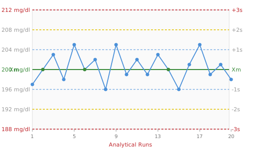
Figure 2 – Chart for total cholesterol
The Levey-Jennings graph is a simple graphical way of plotting the results of repeated analyzes of a known material, called Control Material. It can be understood as a representation of the Gauss curve, if it were rotated by 90 degrees, as represented in figure 2. The values obtained from the analysis of the material on the bench are successively displayed on the graph. Values further away from the Xm line are indicators of greater variation in the method, that is, of increased imprecision.
The distribution of values obtained in the analyzes follows the so-called normal distribution. Results are expected to fluctuate around the average in predictable occurrences, as follows:
- 68.26% of the time will be in the range of ± 1 SD
- 95.46% of the time within ±2 SD
- 99.73% of the time within ±3 SD
In healthcare, it is common to work in the so-called 95% confidence interval (error < 0.05). For this value we will find the range of +– 2 SD in the Gauss curve. It is worth saying that the control results will fall within this range 95% of the time, under stable analytical system conditions. In a still stable system, it is expected that some values will occur outside this range, but still smaller than 3 SD, about 5% of the time. A value between 2 and 3 SD, cannot be considered an error or rejection, but only an alert3.
Parameters for the control chart
The multiple lines represent standardized distance number of standard deviations (SD) above or below the mean, Xm, which is represented by the green line. The blue line is ±1 SD away, the yellow line is ±2SD away, and the red line is ±3SD away. The model is simple and of great value for monitoring measurement processes. Everyone can plot the Levey-Jennings graph, using, for example, graph paper, or using electronic spreadsheets. However, this is far from practical and today we can achieve better results with computational tools.
The green line is central and by convention the average line, at the value in use as a reference for the graph. It is central also because average is a measure of central tendency. It is represented by Xm and can initially be the value provided by the manufacturer of the control material. It is quite possible that the laboratory's own average value is different from the manufacturer's average. If it is very different for a given analyte, the Quality Manager must analyze the results of the Proficiency Tests (External Quality Control) to check the accuracy of that analyte.
For the SD parameter, sometimes represented as 's', from the English standard deviation, which is a measure of dispersion, of random error, we must be even more careful. It is advisable to use the value provided by the manufacturer of the control material (label value), only when conducting a first phase of analyzing the batch of material, which can be called the preparation phase. It is at this stage that the laboratory calculates the proper values for mean and standard deviation, also checking the Coefficient of Variation (CV).
Consider that many manufacturers deliver their leaflets with a variation range and not the SD value. For manual IQC methods, the professional compares the result of the control obtained on the bench with the two values in this range. It's very practical, but it's quite inefficient. It is not a good Internal Quality Control practice because it has a low error detection rate. Furthermore, it is known that manufacturers tend to provide very wide ranges. Therefore, the comparative analysis of the result by range is of low sensitivity in detecting problems and results in incomplete results. It's difficult to talk about quality control. Electronic systems do not use range as a parameter, but objectively use the SD value and provide more information.
We emphasize that to use each new batch of material, the laboratory must establish its own parameters for that batch, carrying out at least 20 analytical runs, in no shorter period
than 10 days. The objective is to obtain the SD value that will be used to demarcate the limits of the Levey-Jennings graph. We call this phase the “Preparation Phase”. After executing this phase and obtaining the mean and SD values, it is recommended to adopt these values as parameters in the control chart, perform a visual analysis and test multiple rules. This second phase is called the "Assets Phase" and represents the moment of indications for acceptance, or the performance of the analytical system.
The need to carry out the preparation phase before actually testing the rules means that many professionals try to obtain all the control material from the same batch from the supplier, with a perspective of duration (consumption time) for at least six months. Ideally, it should be for a year. The longer time is a saving factor, because it eliminates having to carry out preparation phases very often.
Example of control chart interpretation
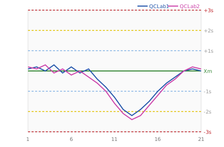
Figure 3 — Graph interpretation for two control levels (QCLab1 / QCLab2)
1. That the average values were below that indicated by the supplier of the control material, since the results fluctuated below the Xm line (green line), around 1 standard deviation.
2. That the oscillation was of small amplitude, indicating a CV smaller than that calculated by the manufacturer's values, which was good.
As the objective was to establish the laboratory's own mean and standard deviation parameters, these values were initially considered acceptable.
The most important aspect was the perception of the trend, of the analytical run from 9 to 15. It indicated a systematic error, which led the analyst to investigate the cause. He understood that the most likely cause would be deterioration of the reagent. The reagent lot was changed and the controls were retested. The results of run 16 and following were considered approved and the values returned to the levels before the deterioration, although still different from the Xm value offered by the manufacturer.
The interpretation of the control chart made a great contribution to detecting deterioration in the system, still in the preparation phase, that is, without yet applying the control rules. Measurements were made (analysis of control materials), application of statistics, plotting and analysis of the graph and the realization that there was a problem. From then on, the decision was made to change the reagent, perhaps considering the history of this analyte and reagent. The run was discarded and the controls were re-analyzed. He concluded that the analytical system recovered the desired balance.
In these actions we can see the last three phases of the PDCA cycle. The analyst carried out Quality Management, based on measurements of the controls and indicators that supported his decision making. It was also evident that in the
Internal Quality Control is true of Peter Drucker's maxim: what is not measured, cannot be managed. Here it was well measured and management provided decision and effective action.
Analysis by multiple internal control rules
Multiple quality control rules, also called "Westgard Rules" (James O. Westgard, PhD)5, represent one of the broadest and most elegant approaches to detecting control problems. They use a set of decision criteria to identify whether an analytical run is in control, or out of control. They are generally applicable with two to four control measures per run, which is to say, with two to four levels of control. In biochemistry, two levels are generally applied with good results for most analytes.
The use of multiple rules must take place after the initial phase – preparation phase – of testing a new batch of control material, based on the Xm and SD values determined in the laboratory itself, in that phase. In this way, the efficiency of multiple rules, both for detecting errors and for avoiding false rejections, becomes notable, aiming to detect possible losses of stability in analytical systems.
We have seen that the application of multiple rules in internal control is easy if a computer system is used. Doing the work manually is more difficult. The use of electronic spreadsheets in Internal Quality Control, such as Excel®, is an alternative adopted by many analysts, but we know that those who use it cannot deal well with the avalanche of difficult-to-manage data, even worse, to carry out all the calculations for many analytes. This form also entails restriction and removal of other members of the laboratory team, who do not have many
times knowledge of the rules and the Excel® program for daily practice. It is very important to fully engage the staff working on the bench, for better results from all quality control actions. We advocate the use of a dedicated computer program, which is even better than the QC modules of analyzer equipment for several reasons. There are now free online programs that offer tests using multiple rules and plotting the Levey-Jennings graph.
It is very important that quality planning considers when applying multiple rules, that there is no one rule, or a set of rules that must be applied to all tests, indiscriminately. Some methods have better precision than others and it is reasonable to apply a different set of rules to them than to others. On the other hand, some tests may require different control requirements and therefore fewer rules are necessary.
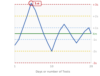
Figure 4 — Rule 1:3s
We describe in detail each of the most common rules, in another available document, "Multiple Rules – Overview of Westgard Quality Control Rules". We suggest you consult it.
The Z value
The computer systems perform various calculations when evaluating the IQC and return the greatest amount of auxiliary information to the user. This adds value to IQC. From these calculations, the systems obtain the Z value, which represents the amount of SD existing from the average, for more or less6. So it will always have a positive value. For the Levey-Jennings graph and for applying multiple rules, the Z value is considered, hence its importance.
For example: For total cholesterol, the average value for use in the Levey-Jennings chart and for applying the rules is 200 mg/dl and the SD is 4.5 mg/dl. The analytical run provided a value of 209 mg/dl. The Z value will then be equal to 2 (209 – 200 = 9; 9/4.5 = 2).
The computer programs display the Z value to the user, that is, how many SD are contained in the dispersion of that run value, which also represents the amplitude of the dispersion. The greater the Z value, the greater the dispersion, that is, the imprecision.
Coefficient of Variation Comparison with Maximum imprecision Values
The performance characteristics of an analytical system that are important for planning quality procedures are imprecision (random error) and bias. It is essential to critically analyze the performance of the analytical system to identify opportunities to improve measurement quality to obtain lower values for random error, reducing imprecision and bias, reducing systematic error9. The assessment of imprecision is part of the scope of Internal Quality Control and has been the subject of this work. Bias will not be addressed here, as it is beyond the scope.
The measure of imprecision can be given by the Coefficient of Variation (CV), calculated by the formula CV = SD / Xm
* 100. It is expressed as a percentage and provides a good estimate of the performance of the analytical method, regarding variability. The mean is a measure of central tendency and is related to accuracy, or the situation of systematic errors. The SD reflects the widening of the distribution of measured values and relates to imprecision, or random errors. The SD will be greater depending on the concentration of the analyte measured in the control material5. It is expected that the SD for level 1, with a mean value in the method's reference range, is smaller than the SD for level 2, with a generally high value, at the pathological level. As the CV reflects an index of the SD and mean, it is a better expression of imprecision for different concentrations and can be used for comparisons.
The CV can be used to compare the performance of one laboratory and another, in a specified method. The CV will be smaller, the smaller the variation in the control results, that is, there will be less imprecision5.
The worst case scenario for errors in the laboratory is given by the Total Error, which represents the combination of the systematic error (bias) and the random error (imprecision) estimated for a method and being in the same direction. Taking care only of imprecision, the lower the CV of the method, the better, because there is "left" more room for systematic error, before compromising the final quality of your result. Therefore, it is an interesting goal for the laboratory to achieve the use of a method that provides a reasonable CV, lower than the maximum desirable imprecision published in the literature2.
The work of Ricós et al. It is very important for consultation by the laboratory, for reference of imprecision. It offers a very valuable table, with numerous tests and values for Maximum imprecision and Total Error, among others. Many laboratory professionals are using this data as a reference, especially for comparing their CV result with the Maximum imprecision value. The goal is to work to get the CV to be less than the published value for Maximum imprecision.
Conclusion and Additional Features
Quality in the laboratory is a function of broad and often complex approaches. In this work we seek to emphasize analytical quality, from three perspectives. It's not everything, but it's an important step, because it can bring to the surface errors that are often obscure, unapparent. Debating them is a notable opportunity for Brazilian clinical laboratories.
Bibliography
- Basques, JCA. Using Controls in the Clinical Laboratory. Labtest Diagnóstica, 2009.
- Ricos, C. et al. Current databases on biological variation: pros, cons and progress. Scand J Clin Lab Invest 1999; 59:491-500.
- Ricos, C et al. Biological variation database, and quality specifications for imprecision, bias and total error. The 2008 update http://www.westgard.com/guest36.htm
- CLSI C24-A3. Statistical Quality Control for Quantitative Measurement Procedures: Principles and Definitions; Approved Guidelines–Third Edition. Clinical and Laboratory Standards Institute, 940 West Valley Road, Suite 1400, Wayne, PA, USA, 2006.
- Westgard JO et al. Basic QC Practices 3rd ed. Madison WI:Westgard QC, 2010.
- Fraser CG. Generation and application of analytical goals in laboratory medicine. Ann Ist Super Sanita. 1991;27(3):369-75.
- Klee GG. Performance goals for internal quality control of multichannel haematology analyzers. Clin Lab Haematol. 1990;12 Suppl 1:65-74.
- Petersen PH, Fraser CG, Jørgensen L, Brandslund I, Stahl M, Gowans E, Libeer JC, Ricós C. Combination of analytical quality specifications based on biological within- and between-subject variation. Ann Clin Biochem. 2002 Nov;39(Pt 6):543-50.
- Basques JCA. Analytical quality specifications. Labtest Diagnóstica, 2009.
- Fraser CG, Harris EK. Generation and application of data on biological variation in clinical chemistry. Crit Rev Clin Lab Sci 1989;27:409-37.
Published May 2012